Developmental xenocortication using human-derived organoids in mice – Nature

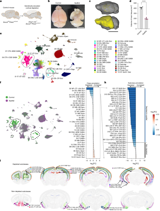
Genetically encoded cortical depletion

Emx1-cre (JAX, B6.129S2-Emx1tm1(cre)Krj/J), Esco2^fl/fl (JAX, B6N.129S-Esco2tm1.1Ge/J) and C57BL SCID (JAX, B6.Cg-Prkdcscid/SzJ) mice were used to generate the breeding scheme: male Esco2^fl/flPrkdc^scid/scid × female Emx1-cre^+/−Esco2^fl/+Prkdc^scid/scid. Breeder and offspring cages were supplemented with breeder chow (Envigo Teklad 2919) and DietGel 76A (with plant protein) to help to increase pup survival. Some breeders were more prone to parental infanticide. In these cases, we implemented an aunting strategy with Swiss Webster active dams from Charles River. To reduce competition for maternal care and milk, a subset of pups was euthanized during the second postnatal week.

hiPS cells, generation of hCOs and viral infection

We generated and cultured hCOs from hiPS cells as previously described^53,54. In brief, hiPS cells were treated with Accutase (Innovate Cell Technologies, AT-104) at 37 °C for 7 min to dissociate them into single cells. The resulting single-cell suspension was collected in a 50-ml Falcon tube, and a cell pellet was obtained by centrifugation at 200g for 4 min. After resuspending the cell pellets, cell counting was performed. Approximately 3 × 10⁶ cells in Essential 8 medium (Life Technologies, A1517001) supplemented with the ROCK inhibitor Y-27632 (10 μM; Selleckchem, S1049) were added to each well of the AggreWell 800 plate (StemCell Technologies, 34815). The plates were then centrifuged at 100g for 3 min to capture the cells in the microwells and incubated at 37 °C with 5% CO₂ (day −1). Then, 24 h after cell aggregation (day 0), spheroids were collected from each microwell by gently pipetting the medium up and down using a cut P1000 tip and transferring them into ultra-low attachment plastic dishes (Corning, 3262) in Essential 6 medium (Life Technologies, A1516401) supplemented with dorsomorphin (2.5 μM; Sigma-Aldrich, P5499) and SB-431542 (10 μM; Tocris, 1614). From days 2 to 5, the Essential 6 medium was changed daily and supplemented with dorsomorphin and SB-431542. On the sixth day in suspension, the neural spheroids were transferred to neural medium composed of Neurobasal A (Life Technologies, 10888), B-27 supplement without vitamin A (Life Technologies, 12587), GlutaMax (1:100, Life Technologies, 35050) and 10 U ml⁻¹ penicillin–streptomycin (Gibco, 15140122). From days 6 to 24, the neural medium was supplemented with 20 ng ml⁻¹ epidermal growth factor (EGF; R&D Systems, 236-EG) and 20 ng ml⁻¹ basic fibroblast growth factor (FGF; R&D Systems, 233-FB), with medium changes occurring daily from days 6 to 15 and every other day until day 24. From days 25 to 42, the neural medium included 20 ng ml⁻¹ brain-derived neurotrophic factor (BDNF; Peprotech, 450-02) and 20 ng ml⁻¹ NT-3 (Peprotech, 450-03), with medium changes every other day. Starting from day 43, the hCOs were cultured in neural medium without growth factors, with medium changes every 4 days.

For viral labelling, all organoids were infected at least 1 week before transplant, most commonly between day 35 and day 40 of differentiation. Organoids were transferred to a 1.5 ml microcentrifuge Eppendorf tube containing 100 μl neural medium with lentivirus and incubated overnight. The next day, neural organoids were transferred into fresh neural medium in 24-well ultra-low-attachment plates with fresh medium changed daily to wash out any ambient virus particles. All lentiviruses were generated by VectorBuilder with previously used vector maps and published sequences: pLV-hSYN1-GCaMP8s, pLV-hSYN1-oScarlet and pLV-hSYN1-eYFP^55,56. For rabies tracing experiments, day 47 hCOs were co-infected with AAV-8-CAG-FLExOFF-RabiesG (AAV-G) from the Stanford viral vector core and G-Deleted Rabies-eGFP (RVΔG-GFP) from Salk Institute. Each organoid was incubated overnight with 0.5 μl of 1:10 diluted RVΔG-eGFP virus and 0.5 μl of AAV-G into 200 μl of the neural medium described above. The next day, 800 μl of the neural media was added to each organoid and, the day after that, the organoids were washed with fresh neural medium three times and transferred into low attachment dishes (6 or 24 well). All cell lines tested negative for mycoplasma contamination, and genomic integrity was assessed using the single-nucleotide polymorphism microarray GSAMD-24v2–0.

Organoid transplantation

All procedures were performed in accordance with NIH guidelines and with previous approval of the Stanford University Administrative Panel on Laboratory Animal Care (APLAC) and in accordance with a previously published protocol¹³, but optimized for the apallial mouse neuroanatomy. In brief, organoids at 30–60 days in vitro were transplanted into 5–17-day old apallial pups (median, 10; interquartile range, 9–13). Importantly, this is before the critical period of activity-dependent establishment of neural connectivity in the mouse⁵⁷. Mice were anaesthetized with isoflurane (5% induction, 2–3% maintenance) and received Ethiqa-XR (0.65 mg per kg) or 10 mg per kg carprofen + 0.25–0.5% bupivacaine local infiltration below the incision site before placement into a stereotaxic frame with a neonatal insert (RWD) and heating pad. Switching from Ethiqa-XR to bupivacaine + carprofen helped to reduce the rate of infanticide. While maintaining an intact dura, a craniotomy was performed on each hemisphere at AP, +1 mm; ML ± 1 mm. For each hemisphere, two hCOs were loaded into the Hamilton syringe and the contents of the syringe were deposited at a rate of 10 µl min⁻¹ at a depth of 1.5 mm below the surface of the dura. This yielded four transplanted hCOs per mouse. As the surgeries occurred at such a young age, there was not enough time to reliably obtain genotyping results before the surgery. Therefore, the presence or absence of the neocortex was confirmed through visual inspection after an initial incision.

MRI monitoring of graft development

MRI scans were performed on the Bruker BioSpec 70/40 small-animal scanner (7.0 Tesla, 300 MHz; Bruker) equipped with a BGA-12S gradient insert (660 mT m⁻¹, 4,570 T m⁻¹ s⁻¹) and interfaced to ParaVision 360 V 3.6. A 4-element receive-only mouse CryoProbe and 86 mm volume coil were used for MR imaging. Animals were anaesthetized with 3% isoflurane mixed in O₂ and maintained with 1–1.5% isoflurane during the imaging procedure. Core body temperature was maintained at 37 °C using a warm water circulator pad and a temperature controller (Thermo Fisher Scientific). Mouse respiratory rates were monitored through a pneumatic pad placed underneath the animal (SA instruments).

Two-dimensional T2W Turbo rapid acquisition with relaxation enhancement (RARE) sequence was used to obtain transverse structural MRI for volume measurements (TR/TE = 4,500/41 ms, FOV = 18 × 18 mm², matrix = 258 × 258 yielding 70 × 70 μm² in-plane resolution, slice thickness = 0.5 mm, RARE Factor = 8, NEX = 2, scan time = 4 min 3 s). For some animals, 3D RAREvfl sequence was used (TR/TE = 1,800/90.26 ms, FOV = 15 × 15 × 8 mm³, matrix = 150 × 150 × 80 yielding 0.100 mm isotropic resolution, RARE Factor = 43, NEX = 1.6, scan time = 10 min 33 s with compressed sensing) and data are reconstructed using the Smart Noise Reduction option.

Two-dimensional SWI data were acquired (TR/TE = 858.8/18 ms, FOV = 15 × 15 mm², matrix = 280 × 280 yielding 54 × 54 μm² in-plane resolution, slice thickness = 0.5 mm, NEX = 6, scan time 21 min 54 s). The volume of brain tissue was determined by segmenting the whole brain and subtracting the volume of cerebrospinal fluid. All analyses were performed with Slicer3D.

For high-resolution anatomical T2W images for DWI co-registration, two RARE sequences were acquired per animal: (1) a low-resolution scan (200 × 200 × 500 µm³) for co-registration reference; and (2) a high-resolution scan (100 × 100 × 300 µm³; RARE factor = 4, TR/TE = 4,000/30 ms, 2 averages, flip angle = 180°) used as the primary anatomical reference for visualization and registration. DWI data were acquired with a four-segment diffusion-weighted EPI sequence (Bruker:DtiEpi) using the following parameters: b = 1,000 s/mm², 40 non-collinear diffusion-encoding directions plus 5 b = 0 images (45 volumes total), diffusion timing δ/Δ = 4.5/10.3 ms, TR/TE = 3,500/21 ms, in-plane resolution 150 × 150 µm², slice thickness 500 µm, FOV = 16 × 15 mm², matrix = 107 × 100, bandwidth = 250 kHz, second-order B₀ map shimming, three FOV saturation bands. The B₀ map was obtained before the sequence and first- and second-order shims were applied using mapshim. NiFti formatted data were converted from Bruker ParaVision format using dcm2niix⁵⁸.

Diffusion-weighted image processing

All diffusion and anatomical data were preprocessed using MRtrix3 (v.3.0.3)⁵⁹ and ANTs (v.2.3.5)^60,61. The processing pipeline was applied identically to all 12 mouse brains. The other analyses were implemented in Python (version ≥3.10) using NumPy⁶², SciPy⁶³, scikit-learn⁶⁴, nibabel⁶⁵ and matplotlib⁶⁶.

Orientation standardization

Raw images were reoriented to match the Allen Common Coordinate Framework (Allen CCF) through a two-step transformation (we called this step flip): (1) axis permutation (axes 2, 1, 0) to map scanner axes to AP, DV and ML axes; and (2) a flip along axis 1 (Y) to align the DV direction with the atlas convention. The same transformation was applied to the 4D DWI data (axes 2, 1, 0, 3) and the high-resolution T2W image.

Preprocessing

We preprocessed all mice with the same protocol using the following steps. (1) Gradient verification: the diffusion gradient table was checked and corrected for orientation consistency using MRtrix3’s dwigradcheck. (2) Denoising: thermal noise was removed using MP-PCA denoising⁶⁷ with a 5 × 5 × 5 voxel kernel and the Exp2 estimator. (3) Brain mask estimation: an initial brain mask was created from the denoised DWI data using dwi2mask, with all automatically generated masks then requiring manual editing. A refined brain mask was manually created from the registered DWI data for use in all downstream analyses. (4) Bias field correction: B₁ field inhomogeneity was corrected using the N4 algorithm from ANTs (B-spline fitting distance = 200, convergence [10, 1e-6], sigma = 4). (5) DWI-to-T2W registration: the bias-corrected mean b = 0 image was rigidly registered to the high-resolution T2W anatomical using ANTs. The resulting affine transform was converted to MRtrix format and applied to the full 4D DWI volume, bringing all diffusion data into T2W anatomical space.

ROI definition

For control mice, the isocortex region of interest (ROI) was derived from the Allen CCF atlas (Allen Institute for Brain Science). The Allen average template was nonlinearly registered to each mouse’s T2W image using ANTs SyN, and the warp was applied to the Allen annotation volume using nearest-neighbour interpolation. ROIs were extracted by collecting all descendant structure IDs under the following parent structures: isocortex (ID 315). Each ROI was split into left and right hemispheres along the midline of axis 2.

For apallial and XCX mouse groups, the apallial cavity or graft, respectively, was manually segmented in 3D Slicer on the high-resolution T2W images. Manual ROIs were transformed with the same flip as the rest of the MRI images and resampled to FOD space using nearest-neighbour interpolation.

FOD estimation

For cross-subject comparability, response functions were averaged across all 12 subjects to create group-level response functions. FODs were then estimated per mouse using multi-shell multi-tissue constrained spherical deconvolution (MSMT-CSD)⁶⁸ with the group-averaged WM and CSF response functions. Intensity normalization was performed using mtnormalise⁶⁹ with WM and CSF compartments only (three-tissue normalization including GM was unstable for mouse brain data). The resulting group-normalized WM FOD images were used for all subsequent analyses. As a negative control, we confirmed the lack of directional FODs in the apallial cavity and excluded the apallial group from statistical comparisons between groups.

Fixel-based analysis

FODs were decomposed into discrete fixels using fod2fixel, yielding per-fixel apparent fibre density and peak amplitude maps. The voxel-wise total apparent fibre density was computed by summing all fixel contributions through fixel2voxel. Directional fibre density within each ROI was decomposed into AP, DV and ML components for ROI-level microstructural characterization.

Slicewise fixel direction analysis

To characterize the spatial organization of fibre orientations within the seed ROI, a slicewise fixel analysis was performed. For each coronal slice through the seed ROI (isocortex for control, graft for XCX), fixel peak direction vectors were extracted from the group-normalized FOD using fod2fixel followed by fixel2peaks. Fixel directions were clustered into two populations using k-means clustering (k = 2) applied to the absolute values of the direction vectors (to handle antipodal symmetry). For each cluster, the mean direction was computed using the scatter-matrix eigenvector method, which correctly averages axial data by finding the principal eigenvector of the covariance matrix, \(S=\sum _{i}{v}_{i}{v}_{i}^{T}\). Cluster directions were scaled by the mean FOD peak amplitude to produce amplitude-weighted direction vectors.

Voxel-wise dominant diffusion orientation

For each voxel, the primary direction of restricted water diffusion (defined as the fixel corresponding to the largest FOD lobe) was identified. The spatial orientation of this dominant diffusion component was categorized by the axis with the largest absolute component of its direction vector (AP, DV or ML). The percentage of voxels dominated by each spatial direction was calculated per subject and averaged per group.

Direction vector r.m.s.d. analysis

Within-group consistency of fibre orientations was quantified by the r.m.s.d. of direction vectors across mice, computed per slice and overall:

where v_i is the k-means cluster 1 direction vector (scaled by FOD peak amplitude) for subject i, and \(\bar{{\bf{v}}}\) is the group mean vector. The mean vector norm \(\Vert \bar{{\bf{v}}}\Vert \) and the ratio \(\frac{{\rm{r.m.s.d.}}}{\Vert \bar{{\bf{v}}}\Vert }\) were also computed to contextualize variability relative to signal magnitude.

Radar plots

Fixel direction vectors were visualized as radar (polar) plots with three axes corresponding to the AP, DV and ML anatomical directions. Each radar plot displays one coronal slice through the seed ROI. A thin radial grid with three concentric rings provides the amplitude scale. The amplitude axis was unified across all groups and slices for direct comparison.

Whole-brain tractography

Whole-brain tractograms were generated using the iFOD2 probabilistic algorithm⁷⁰ seeded from the brain mask. Tracking parameters were as follows: step size = 0.02 mm, maximum angle between successive steps = 60°, FOD amplitude cutoff = 0.1, minimum streamline length = 2 mm, maximum streamline length = 15 mm. 1 million streamlines were generated per subject.

Rabies-virus-based monosynaptic retrograde tracing from organoid graft

hCOs were pre-infected with Rb-GFP and AAV-G as described above, washed multiple times with fresh medium followed by daily medium change for 3 days and transplanted as described above. Then, at 3 weeks after transplantation, the mice were transcardially perfused as described above. Deletion of the rabies-virus G gene restricts retrograde transport to cells carrying the G protein (that is, one retrograde step from the organoid). The entire forebrain was sectioned (100 µm) into four series (300 µm space between sections) and individual series were mounted. The series of sections used for analysis were also immunostained with HNA and only HNA⁻GFP⁺ cells were included for analysis. Sections consecutive to the analysed series (that is, the next series) were immunostained for TH and PV to reveal the CP and reticular thalamus (respectively) to aid identification of regions. Then, using the Allen Institute Brain Atlas, bright-field images of the sections revealing white matter tracts, previous MRIs of apallial mice and the TH and PV immunostaining, we localized each section for analysis to the relevant AP slice in the brain atlas. Then, using the BigWarp plugin for FIJI/ImageJ⁷¹, we warped the atlas to relevant anatomical landmarks. Finally, we manually counted HNA⁻GFP⁺ cells using the CellCounter plugin within the defined brain regions. Owing to the altered anatomy in the apallial mouse, here we combined subregions into Allen Institute’s classification of parent structures. Cells in regions that could not be reliably delineated, as well as a small number of midbrain inputs, were included in the total input count but not shown as separate regional categories. Accordingly, the regions presented accounted for 98.1–100% of labelled inputs per animal, and percentages do not necessarily sum to 100%.

MoSeq analysis

Behavioural data acquisition was performed similar to previous descriptions. Mice were tested in a circular open-field arena (18 inch diameter, 15 inch height; US Plastics) under dim red illumination. The opaque enclosure was spray-painted black (Acryli-Quik Ultra Flat Black) to avoid image artefacts. Each animal was placed into the centre of the arena and allowed to explore freely for 60 min. Between trials, the enclosure was wiped sequentially with 10% bleach, 1% Alconox and 70% ethanol to remove odour cues. All sessions were run during the dark phase, when mice are naturally active. 3D tracking was obtained using the Microsoft Kinect v2 depth sensor mounted approximately 65 cm above the arena to give a top-down view. Depth frames were streamed at 30 Hz over USB 3.0 to a dedicated acquisition computer (Intel i5-6400 CPU, 16 GB RAM, NVIDIA GT1030 GPU) and written to disk in raw binary format via a custom C#/C++ interface.

Analysis of MoSeq

Preprocessing and modelling with MoSeq

All depth videos were processed with the open-source MoSeq pipeline (Python) running either on local workstations or on the Stanford cluster computer (Sherlock 2). Each raw frame was first resampled and background-subtracted using a median depth image built from the initial 1,000 frames. Negative values and pixels higher than the defined ceiling were zeroed, yielding a clean relief map of which the intensities represent the height above the arena floor. The mouse contour was located, its centre of mass and yaw angle were computed, and an 80 × 80-pixel patch centred and aligned to the nose–tail axis was extracted for every frame. The resulting 30 Hz image stack constitutes the aligned behavioural video.

For modelling, every stack was flattened and reduced by PCA. The principal component time series from all animals of a sex were then whitened to remove cross-component covariance. Separate autoregressive hierarchical Dirichlet-process HMMs (AR-HMMs) were fitted to the male and female datasets. Each model was truncated after the first 60 latent states (syllables), which together accounted for at least 99% of the total variance, and these state sequences formed the basis of all downstream analyses.

Behavioural summaries

Session-level behavioural fingerprints were assembled by concatenating four kinematic distributions with a truncated syllable-usage vector. As previously described, the distance of the animal’s centre to the arena centroid and its planar speed were each binned into 100 equiprobable intervals, whereas body height and body length were summarized with 45-bin histograms. The syllable component comprised the relative occupancy of the first 60-syllable labels produced by sex-specific AR-HMMs. Histograms were normalized such that every column represented a probability distribution. Scalar channels were additionally scaled to a common 0–1 range using the global minimum and maximum estimated across sessions of the same sex. For downstream analyses, the four scalar histograms and the syllable vector were stacked to yield a 350-element feature vector per recording session (2 × 100 + 2 × 45 + 60). The resulting matrix (sessions × features) constitutes the behavioural summary used for all classification and statistical tests.

Classification and confusion matrices

Linear classifiers were trained independently on each feature modality—distance to centre, planar velocity, body height, body length and the 60-element MoSeq vector—using the session-level fingerprints described above. For a given modality, the relevant column(s) were extracted from the fingerprint matrix, concatenated into X, and paired with the session label y (CON_SES1 and so on). A one-versus-rest logistic-regression model (liblinear optimizer) served as the base estimator. The penalization constant C was optimized once, before cross-validation, by a grid search over 50 logarithmically spaced values between 10⁻⁶ and 10³.

Performance was assessed with 500 repeated stratified shuffle–split resamples that preserved class proportions (80% training, 20% test per fold). Each split was processed in parallel across CPU cores; within every split, the model was fit to the training set and evaluated on the withheld samples. To obtain a chance-level baseline, the entire procedure was repeated 100 times with the class labels randomly permuted before fitting. The resulting collections comprise, for every modality, the vectors of true and predicted labels, the per-split coefficient vectors and overall accuracies for both the real and the shuffled runs; they were serialized for reproducibility. The displayed matrices and accuracy labels summarize the original 500 session-level splits, with C selected on the full dataset and without grouping by mouse. An additional sensitivity analysis used 500 80:20 splits of mice, stratified by experimental group, with all sessions from each mouse kept together. Within each training set, C was selected by threefold mouse-grouped cross-validation over the same grid, keeping the cohort-derived features fixed. Pooled held-out accuracies for MoSeq, speed and position were 0.590, 0.351 and 0.311 in males and 0.631, 0.490 and 0.440 in females, respectively.

Aggregated predictions were summarized as row-normalized confusion matrices (i,j) whose entry gives the fraction of samples from true class iassigned to class j. For each modality, the real and shuffled matrices were displayed side by side, rendered on a 0–1 greyscale.

Held-out confusion analysis

To assess pairwise similarity between behavioural conditions without relying on any within-class information, we performed a leave-one-class-out evaluation on the syllable-usage fingerprints. For each sex, the 60-dimensional MoSeq vector of every session was retained, row-normalized to unit sum and associated with its class label (CON_SES1 and so on). The procedure iterated once over every label: at each iteration all sessions belonging to the target class were withheld as the test set, a linear logistic-regression model with L2 regularization (inverse-variance class weighting, regularization constant = 100, liblinear optimizer) was fitted to the remaining data and immediately applied to the unseen samples. Concatenating the predictions from all iterations yielded a square confusion matrix (i,j) of which the entry recorded the proportion of samples of true class i classified as j after row normalization. The matrix was visualized with a perceptually uniform greyscale and the standard group/session colour palette, providing an intuitive map of interclass similarity that is independent of cross-validation performance metrics.

F-statistics for syllable-level discrimination

As previously described, we identified the syllables that contributed most strongly to group differences by applying a univariate F test to the row-normalized MoSeq usage matrix. For each sex, the 60-element usage vector of every session was first normalized to sum to one. Two contrasts were then evaluated independently. In the one-versus-rest contrast, every class was compared with the pooled remainder; in the session-matched control contrast, each treatment session (APA_SES1, APA_SES2, XCX_SES1, XCX_SES2) was tested against the control session with the same session number (CON_SES1 or CON_SES2). For a given contrast, the labels were converted to a binary vector and, for every syllable, an F statistic and corresponding P value were obtained with the f_classif implementation in scikit-learn. Syllables of whose tail probability multiplied by the number of tested syllables fell below 0.01 were deemed to be significant. For every class, the full vector of F values, the associated P values and the indices of significant syllables were saved. These outputs were visualized as horizontal barcode plots in which each strip shows the F statistic normalized to its class-specific maximum, and the number of significant syllables is indicated in the legend.

Linear-discriminant embeddings and distance metrics

Syllable-level embeddings were derived with LDA. For each sex, the per-session MoSeq fingerprint was reduced to the 60-dimensional, row-normalized syllable-usage vector. These vectors were assembled into a sessions × syllables matrix and supplied, together with the categorical label denoting either the experimental group (control, apallial, XCX) or the full group-by-session identifier (for example, apallial-2), to an LDA model with two components for the experimental-group labels and three components for the group-by-session labels, using the eigen-solver with automatic Ledoit–Wolf shrinkage. The resulting coordinates were visualized as 2D and 3D scatter plots coloured according to the palettes used throughout the study.

Session-pair distances were computed in LDA space as the Euclidean norm between the embeddings of the first and second recording session of each mouse. Only mice contributing both usable sessions were included. Distances were summarized by grey bars showing the mean ± s.e.m. overlaid with jittered points for individual animals. Group differences were evaluated using a Kruskal–Wallis test followed, where appropriate, by pairwise two-sided Mann–Whitney U-tests with Bonferroni correction.

To relate treatment trajectories to the baseline behaviour, we calculated, for every XCX mouse session, the distance in LDA space to the combined centroid of control mouse sessions and to the combined centroid of apallial mouse sessions. Repeated sessions were first averaged within each reference mouse, and the reference centroid was then calculated across mice so that every reference mouse contributed equally. The two distances for each XCX mouse and session were compared using a two-sided Wilcoxon signed-rank test, and the resulting P values were Bonferroni corrected across the two embedding metrics and two sessions within each sex.

KLD analysis

Behavioural-variability metrics were adapted from a previous study³⁴. As in that study, syllable-usage distributions were summarized using KLD and CV. As experimental condition was assigned at the level of the mouse, repeated sessions and derived syllable or mouse-pair values were not treated as independent biological replicates in inferential analyses.

To quantify the within- and between-animal differences in syllable usage, we calculated the KLD between normalized syllable-occupancy distributions. For every mouse, we assembled two distributions—one from the first recording session (SES1) and one from the second (SES2)—each defined over the first 60 syllable labels and regularized with a 1 × 10⁻¹⁰ pseudocount to avoid undefined logarithms. The within-mouse divergence DKL(SES1‖SES2) was obtained by summing p log(p/q), where p and q are the respective occupancy vectors.

Between-animal differences in syllable usage were assessed by first averaging the two sessions of every animal to a single subject-level distribution and then computing the KLD for every unique pair of animals within the same experimental group. To remove dependence on mouse ordering, inter-mouse KLD was symmetrized as D_sym(p,q) = [D_KL(p‖q) + D_KL(q‖p)]/2. Pairwise values were retained for visualization, but statistical inference was performed by permuting whole-mouse group labels while preserving group sizes and recomputing the mean within-group dispersion. Omnibus P values were estimated using label permutations; pairwise P values were obtained from exact two-group label permutations using the absolute difference in mean dispersion and were Bonferroni-corrected for three comparisons.

CV analysis

The coefficient of variation (CV = σ/μ) was used to quantify the spread of syllable-usage probabilities. For the intramouse analysis, a CV was computed separately for every syllable across the two recording sessions, and finite syllable-level values were averaged to yield one value per mouse. Group effects were assessed using a Kruskal–Wallis test followed, when significant, by pairwise two-sided Mann–Whitney U-tests with Bonferroni correction. For the intermouse analysis, the two sessions of each animal were first averaged to a single subject-level distribution, after which the CV across all animals of the same experimental group was calculated syllable-wise. Syllable-level values were retained for visualization. Statistical significance was assessed by permuting whole-mouse group labels while preserving group sizes and recalculating the group CVs on every permutation. The omnibus statistic was the sample-size-weighted between-group sum of squares of the group mean CVs. Omnibus P values were estimated using permutations; pairwise P values were obtained from exact two-group label permutations using the absolute difference in mean CV and were Bonferroni-corrected for three comparisons.

Intra-session differences in syllable usage using window-to-session KLD

The temporal stability of syllable expression within a recording was assessed in overlapping 60 s windows advanced every 30 s. For each session, the framewise syllable labels were converted to a sequence of occupancy histograms (one per window; 60 syllable bins). Windows containing no frames were skipped.

Window histograms were first converted to probability vectors pw by adding a 1 × 10⁻⁹ pseudocount to every bin (to avoid zero probabilities in the KLD calculation) and then normalizing to unit sum. The session-average distribution q was computed across all windows, and the divergence for window w was D_KL(p_w‖q) = Σi p_wi log(p_wi/q_i). The mean KLD over windows yielded a session-level drift index. For the base-group comparisons reported in Fig. 4f and Extended Data Fig. 8o, repeated-session indices were averaged within mouse before inference.

Distributions were visualized as grey bars indicating the mean ± s.e.m. across mouse-level means, with jittered session-level points overlaid for visualization. Group effects were tested on mouse-level means with a Kruskal–Wallis test followed, when significant, by pairwise Mann–Whitney U-tests with Bonferroni correction.

For temporal CV, the CV of each syllable was calculated across the same overlapping 60 s windows, and finite syllable-level CVs were averaged to yield one index per session. Repeated-session indices were then averaged within mouse. Group effects were tested with a Kruskal–Wallis test followed, when significant, by pairwise two-sided Mann–Whitney U-tests with Bonferroni correction.

Temporal stack plot of syllable usage

For qualitative illustration of how behavioural composition evolves over the course of a recording, we generated stack plots that lay out the relative occupancy of each syllable across consecutive, non-overlapping 60 s windows (the same window length as used for the CV and KLD analyses). For a given recording, all video frames falling inside the user-defined time slice (3 s after start to the end of the file) were binned into contiguous 60 s segments; any partial segment at the end of the file was discarded. Within each window the number of occurrences of every syllable label (from 0 to 59) was counted, divided by the total number of frames in the window and clipped to the first 60 labels to match the palette length. The resulting 60 × N matrix, where N is the number of windows, was plotted with matplotlib.stackplot, producing a coloured band for each syllable whose vertical thickness represents its moment-to-moment fractional usage.

Directed behavioural studies

Male and female mice (aged 3–5 months) were used in this study, with organoids 4–5 months after differentiation. Control mice were littermates of apallial or XCX mice but lacked Cre recombinase expression in tail DNA (that is, Esco2^fl/flPrkdc^scid/scid genotyped through Transnetyx). For behavioural testing, mice were group-housed in a Stanford University animal facility under a reversed light–dark cycle (lights off at 08:30 and on at 20:30) with free access to food and water. All directed behavioural studies were conducted during the mouse dark cycle, following a 1 week habituation period to the facility and 3 days of handling. All procedures adhered to National Institutes of Health guidelines and were approved by the Institutional Administrative Panel on Laboratory Animal Care (APLAC). Body weight growth was measured and only mice with body weight recorded at 1, 2 and 3 months of age were included in the analysis. Mice from all conditions were excluded from behavioural analysis if there were systemic morbidities unrelated to transplantation such as paraphimosis or malocclusion.

Open-field activity chamber

The assessment took place in an open-field activity arena (Med Associates, ENV-515) mounted with three planes of infrared detectors, within a specially designed sound-attenuating chamber (Med Associates, MED-017M-027). The arena is 43 cm (L) × 43 cm (W) × 30 cm (H) and the sound-attenuating chamber is 74 cm (L) × 60 cm (W) × 60 cm (H). The mice were placed in the corner of the testing arena and allowed to explore the arena for 10 min while being tracked by an automated tracking system. Parameters including distance moved, velocity, rearing, and times spent in the periphery and centre of the arena were analysed. The periphery was defined as the zone 5 cm away from the arena wall. The arena was cleaned with a 1% Virkon solution at the end of each trial.

Y-maze spontaneous alternation assay

This test is based on the tendency of rodents to explore new environments and alternate arm entries in a Y-shaped enclosure. The arena consists of three plastic arms in a Y shape, including one long arm (A, 20.32 cm × 12.7 cm × 7.62 cm) attached to two shorter arms (B and C, 15.24 cm × 12.7 cm × 7.62 cm), separated by 120°. Mice were placed in the centre of the maze facing the intersection between arms B and C and allowed to freely explore. Using an overhead camera, the number of arm entries and alternations were recorded for 5 min. An entry is recorded when all four limbs of the mouse have entered the arm. The first entry was excluded from data analysis due to potential influence from the experimenter. The Y maze was cleaned with a 1% Virkon solution between mice. After testing, the entries are scored for the number of alternations, defined as any combination of three unique consecutive arm entries (that is, ABC or BAC, but not CAC). The percentage alternation rate is calculated as the number of alternations/the total number of possible alternations × 100. Only mice that performed at least 10 arm entries within 5 min were included in the alternation comparison analysis.

CatWalk

Gait assessment was performed using the CatWalk XT apparatus and CatWalk XT v.10.7 software (Noldus IT). The operation principles of the CatWalk were described previously⁷². During the trial, mice were allowed to walk across the glass platform (dimensions, 40 cm (length), 10 cm (width)) three times in an unforced manner. Runs across the walkway were considered successful only when the run duration was between 0.5 s and 5 s. Only one run per trial was analysed based on duration and continuity of the run. Normal rodents demonstrate three categories of step sequences: cruciate, alternate and rotate. Each category can be broken down into two unique patterns, totalling six observable step patterns. For example, cruciate can be broken down into cruciate A (Ca) and B (Cb). Ca is characterized by the following sequence of paw placements: right front (RF), left front (LF), right hind (RH), left hind (LH). Cb: LF, RF, LH, RH. Aa: RF, RH, LF, LH. Ab: LF, RH, RF, LH. Ra: RF, LF, LH, RH. Rb: LF, RF, RH, LH⁷³. Mice were tested after the AC and Y-maze SA assays. Phase dispersion data are circular, ranging from −50% to +75%. For diagonal paw pairs presented in Fig. 4m, all values fell between −13% and +17%. As the values are far from the −50%/+75% wrap boundary, the circular and linear means of the groups differed by less than 0.05 (for example, 4.323% versus 4.283% for the apallial LF–RH pair). Therefore, a linear two-way ANOVA with paw-pair as a within-subject factor was used.

Three-chamber social-interaction test

The test was conducted using a rectangular plexiglass apparatus (60 cm × 40 cm × 22 cm) divided into three interconnected chambers of equal size (each 20 cm wide). Transparent walls with 5 cm × 5 cm openings allowed the mouse to move freely between chambers. Each outer chamber contained a wire cup (10 cm in diameter, 11 cm height), used to enclose a stimulus mouse or an object. To reduce stress and novelty effects, two unfamiliar stimulus mice (stranger 1 and stranger 2) were habituated to the wire cups for 30 min before testing. The test consisted of three consecutive 10 min phases. In the habituation phase, the mouse was placed into the centre chamber and allowed to explore all three empty chambers freely. In the sociability phase, stranger 1 (a sex- and age-matched unfamiliar C57BL/6 mouse) was enclosed in a wire cup and placed in the right chamber, while a novel inanimate object was placed in a wire cup in the left chamber. The mouse was allowed to explore all chambers, and the time spent interacting with stranger 1 versus the object was scored to assess sociability. In the social novelty phase, stranger 2 was introduced into a new wire cup in the right chamber, while stranger 1 was moved to the left chamber. The mouse again explored the apparatus for 10 min, and interaction times with each unfamiliar mouse were recorded to evaluate social novelty preference. New wire cups were used in each session to eliminate odour cues, and the apparatus was thoroughly cleaned with 1% Virkon between trials. When applicable, mice were tested after the AC, Y-maze SA and CatWalk assays.

Aversive Pavlovian trace conditioning procedure

The Coulbourn Instruments Aversive Conditioning System and FreezeFrame software were used for the aversive Pavlovian trace conditioning assay, which consisted of three phases: training (day 1), contextual testing (day 2) and cued testing (day 2). The training and contextual testing chambers were identical, featuring aluminium walls, a grey metal grid floor (for shock delivery), red house lights and a mint scent to create a distinct context. Chambers were cleaned with a 10% Simple Green solution (Sunshine Makers) between mice. The cued testing chamber was distinct from the training chambers, featuring circular blue plastic walls and flooring, yellow house lights, continuous 80 dB ‘waterfall’ background noise and a vanilla scent. These chambers were cleaned with 70% ethanol between mice. All of the chambers were enclosed in sound-attenuating chambers equipped with mounted speakers, exhaust fans and cameras for behavioural recording. On training day (day 1), the mice were individually placed into the training chamber for 3 min. A tone (20 s, 80 dB, 2 kHz) was played, and a mild foot shock (0.5 mA, 2 s) was delivered 18 s after the tone ended (that is, an 18-s trace period). This procedure was repeated three times with 60 s intervals between shocks. After the final 60 s period, the mouse was returned to its home cage. On contextual testing day (day 2), mice were placed back into the same training chamber for 5 min without any tone or shock to assess their contextual memory. For cued testing (day 2), the mice were placed into the cued testing chamber for 3 min of habituation, followed by three tone presentations (20 s, 80 dB, 2 kHz) at 80 s intervals, without shocks, to assess cue-dependent learning. Freezing behaviour was recorded by an overhead camera and analysed using FreezeFrame software. Freezing was defined as the complete absence of movement for at least 0.75 s, and the percentage of freezing during each phase was measured. When applicable, mice were tested after the AC, Y-maze SA, CatWalk and three-chamber social-interaction tests.

Active avoidance test

The active avoidance test was conducted using the Gemini Active/Passive Avoidance System (San Diego Instruments) to assess associative learning and avoidance behaviour in mice. The apparatus consisted of a two-compartment shuttle box equipped with an automated guillotine door, a stainless-steel grid floor capable of delivering mild foot shocks, built-in speakers for auditory stimulus presentation and overhead lights. The system was enclosed in a sound-attenuating chamber, and all trials were controlled and recorded using Gemini software.

Mice were trained in the active avoidance task over three consecutive days. Each training session consisted of 50 trials per day, totalling 150 trials across the experiment. At the beginning of each testing day, mice are acclimatized for 5 min inside the apparatus and freely allowed to transition between the two compartments. The animal location was detected by the infrared sensors in the compartments. Each trial began with the presentation of the house light for 10 s as the conditioned stimulus (CS) signalling the impending foot shock. If the mouse crossed into the opposite compartment during the CS period, the response was recorded as a successful avoidance, and no shock was delivered. If the mouse failed to cross during the CS, an unconditioned stimulus was administered in the form of a mild foot shock (0.4 mA, 2 s). The shock was automatically terminated after crossing or after 2 s had elapsed. Trials were separated by a variable intertrial interval of 30 ± 5 s.

The numbers of successful avoidance responses (crossing before shock onset), escape responses (crossing after shock onset) and no response (remaining in the same compartment and received 2 s of shock) were recorded for each mouse. Chambers were cleaned with 70% ethanol between animals to minimize olfactory cues. Active avoidance experiments were conducted after aversive Pavlovian trace conditioning.

Hot plate

A hot plate apparatus (IITC, 39) set to 55 °C was used in the study. The mice were placed onto the hot plate and covered by a transparent glass cylinder that was 25 cm high and 12 cm in diameter. A 30 s maximum trial duration was used during the test to minimize the exposure of animals to painful stimuli and prevent permanent tissue damage from the heat. A remote foot-switch pad was used to control the start/stop/reset function. The latency to hind paw licking, flicking or jumping was recorded. The hot plate test was performed after the active avoidance test.

VF filament

The VF test is a method used to assess mechanical sensitivity by applying calibrated filaments of increasing or decreasing force to the skin or paw and measuring the withdrawal response threshold. The VF setup included custom built wire grid flooring (grid size 1.27 cm; 61 cm length × 41 cm width) elevated 61 cm, a clear upside-down 1 l beaker and a set of VF filaments (North Coast, Touch-Test Sensory Evaluator, NC12775). Twelve filament sizes (0.02, 0.04, 0.07, 0.16, 0.4, 0.6, 1, 1.4, 2, 4, 6 and 8 g) were used in the assessment. Mice were habituated to the VF filament test setup for 10 min per day for 3 days before testing. During the testing day, the mouse was habituated under the beaker for 10 min. The test began when the mouse stopped exploring and acclimatized to the testing environment.

The up–down method⁷⁴ was used to determine the mechanical withdrawal threshold of both left and right hind paws. Testing started with the 0.4 g filament. If the mouse did not withdraw the paw, the next higher-force filament was applied. If the mouse did withdraw, the next lower-force filament was applied. This continued until four responses after the first change in withdrawal direction were recorded. The sequence of responses (X for withdrawal, O for no response) was recorded. To ensure accuracy, at least six responses around the estimated threshold were collected. The 50% withdrawal threshold was then calculated using the formula 50% threshold = \({10}^{({X}_{f}+{kd})}\). X_f represents the base-10 logarithm of the force in grams of the final filament used, k is a tabular value based on the response pattern⁷⁴ and d is the difference between the base-10 logarithms of adjacent filament forces. This calculation allowed for a statistical determination of the mouse’s mechanical sensitivity.

Each filament was applied from below the wire mesh to the central plantar surface of the left and right hind paws, avoiding the footpads. The filament was pressed until it slightly bent, maintaining contact for approximately 2 s. To ensure consistency, filaments were applied only when the mouse was stationary and standing on all four paws. A minimum interval of 20 s was allowed between each filament application to avoid sensitization and ensure reliable responses. A withdrawal response was considered valid only if the hind paw was completely lifted off the platform. If the mouse walked away immediately after filament application instead of simply withdrawing the paw, the filament was reapplied. In rare cases in which a mouse flinched but did not fully lift the paw, the response was not counted as a withdrawal. The VF test was performed after the hot plate test.

OEG analysis

Mice were anaesthetized with isoflurane (1–2% in oxygen), and the scalp was surgically removed to expose the skull. The skull surface was cleaned and dried before affixing a custom aluminium head plate using dental cement (C&B Metabond, Parkell) to enable head fixation and provide optical access to the dorsal aspect of the hCO transplant. Finally, the exposed skull was coated with a thin layer of cyanoacrylate adhesive (Krazy Glue, Toagosei America) to render it more optically homogeneous. Widefield fluorescence imaging was conducted using a custom-built tandem-lens macroscope comprising a pair of camera lenses (Nikkor 50mm f/1.2, Nikon) separated by a 499/654 nm dual-band dichroic mirror (499_654 ULTRA, Alluxa) mounted in a 60 mm cage cube (LC6W, Thorlabs). To isolate GCaMP-related signals, emitted fluorescence was band-pass filtered around 520 nm (FF01-520/35-50.8-D, Semrock) before being captured on a sCMOS camera (OrcaFlash 4.0v2, Hamamatsu). For most experiments, the imaged field of view was 13.312 × 13.312 mm² divided into 512 × 512 pixels with a pixel size of 26 µm × 26 µm. To distinguish Ca²⁺-related fluorescence from non-Ca²⁺-dependent artefacts, data were acquired with alternating excitation at 470 nm (Ca²⁺ sensitive) and 405 nm on consecutive frames. GCaMP8s is significantly less sensitive to Ca²⁺ at 405 nm and demonstrates an inverted response. In a subset of high-speed-imaging experiments, a 340 × 340 pixel region of interest covering the implant was recorded at around 142 Hz (7 ms exposure) with constant 470 nm illumination. Widefield imaging data were de-interleaved to separate the 470 nm and 405 nm colour channels. Normalized fluorescence (ΔF/F) was calculated for each channel by dividing each pixel’s timeseries by its mean, subtracting 1, then detrending linearly. The 405 nm channel was low-pass filtered below 14 Hz and regressed pixelwise onto the signal channel. The resulting, artefact-corrected residual signal ΔF/F after regression was used for all further analyses.

The pixel-wise average timeseries across the entire imaged cortical surface was extracted and z-scored. Calcium burst onsets were delineated by finding frames where the temporal derivative of the z-scored cortex-wide activity exceeded a threshold of 0.5 and brain-wide average raw ΔF/F₀ activity exceeded 10% within 10 frames thereof. If multiple nearby frames met this criterion the earliest was used. Burst offsets were defined as the frame at which activity returned to the baseline (<1% of burst peak) and did not spike again for at least 30 s. To examine the tendency of events to recruit the entire cortical surface, we calculated the fraction of pixels participating in each event—where participation was defined as having activity exceeding 3 s.d. above its session-wise mean ΔF/F₀ during the event period—for each technical replicate. A null model of burst participation was then generated by independently shuffling each pixel’s timeseries and recomputing the fraction of pixels whose activity exceeded 3 s.d. above its session-wise mean ΔF/F₀ during the previously defined burst periods. We repeated this shuffling procedure 1,000 times per replicate to generate an estimate of the null probability of burst participation under the assumption that pixels were uncorrelated in their activity.

Visual inspection of the time course of calcium bursts revealed that they often comprised what appeared to be multiple events with several activity peaks occurring in succession, although at variable intervals across mice. To assess the sub-burst dynamics, we used calcium deconvolution to extract the discrete, spike-like events underlying the protracted bursts. The one-dimensional pixel-wise average ΔF/F₀ timeseries was linearly detrended and its minimum subtracted to ensure non-negativity, then deconvolved using the OASIS AR-2 algorithm as implemented in CaImAn to detect events. Interevent intervals were then calculated as the time between events within a calcium burst. Note that the data are quantized to 32 ms due to the acquisition frame rate.

An infrared camera (Basler ace acA1440-220um) was used to record high speed (125 Hz) videos of orofacial motor activity during calcium imaging. The total motion energy was computed as the frame-wise sum of the absolute pixel-wise temporal derivative of the greyscale videos, then normalized between 0 and 1 for each session. Plotting the average calcium and motion energy timeseries across all bursts from all sessions, we found a strong correlation between neural activity and orofacial movement. To quantitatively assess this relationship, we computed the average normalized motion energy during Ca²⁺ bursts and compared this value to that when no burst was occurring.

Acute in vivo extracellular electrophysiology

Mice were briefly anaesthetized with isoflurane, and a craniotomy was opened directly above the cortical locus that mesoscale calcium imaging had identified as the origin of spontaneous activity bursts. The animal was transferred to an air-supported Styrofoam-ball apparatus and head-fixed. A silver-chloride ground/reference wire rested in a saline pool on the skull. A motorized micromanipulator (MPC-200, Sutter Instrument) advanced a 32-channel linear silicon probe (electrode spacing: 40 μm, A1x32-Edge-10mm-40-177-CM32, NeuroNexus) through the craniotomy and into the graft. The shank had been coated with the lipophilic tracer DiI (Thermo Fisher Scientific, D282) to enable subsequent histological verification of the recording trajectory. Neural signals were amplified 10,000-fold, band-pass filtered between 0.1 Hz and 7.5 kHz, and digitized at 30 kHz using an Open Ephys acquisition board coupled to an Intan RHD headstage; data streams were written continuously to disk for offline analysis. To quantify locomotor activity during head fixation, the 20-cm Styrofoam sphere was randomly patterned with 2–5 mm black dots spaced around 20 mm apart. A monochrome GigE camera (Mako U-130B, Allied Vision) captured a 100 px × 150 px region of interest on the sphere at 30 fps throughout each recording session. Frame-to-frame displacements were estimated with an FFT-based phase-correlation algorithm. The resulting x– and y-pixel shifts were converted to physical distances with an empirically determined pixel-to-centimetre calibration factor and divided by the 33.3 ms interframe interval to yield instantaneous speed in cm s⁻¹. All recordings were performed during the light phase.

LFP burst and peak detection in extracellular electrophysiology

Broadband traces (30 kHz) were downsampled to 1.5 kHz. Bursts were flagged by visual inspection as conspicuous epochs of which the envelope exceeded background fluctuations on at least one channel. Within each burst, individual extrema were extracted with scipy.signal.find_peaks using minimum and maximum polarity-specific amplitude thresholds that were empirically adjusted for each session. Detections separated by <5 ms were merged. All peaks were subsequently reviewed and, when necessary, manually corrected by an experimenter. These deliberately conservative criteria were optimized to capture clear, large-amplitude LFP events and, as a trade-off, may have excluded smaller deflections.

Tissue preparation and immunostaining

Mice were deeply anaesthetized and transcardially perfused with PBS followed by 4% paraformaldehyde (PFA). After cryoprotection in 30% sucrose, brains were cryosectioned at a thickness of 50 μm using the Leica CM1860 cryostat. For immunostaining, free-floating tissue sections were washed three times with PBS, then blocked and permeabilized for 1 h at room temperature in PBS containing 0.3% Triton X-100 and 10% normal donkey serum. Primary antibodies were diluted in the blocking buffer and incubated with the sections overnight at 4 °C. After three washes with PBS, the sections were incubated with the corresponding Alexa Fluor secondary antibodies for 2 h at room temperature. The samples were then mounted onto microscope slides using Fluoromount-G Mounting Medium (Southern Biotech).

The primary antibodies used were: anti-CTIP2 (rat, 1:200, ab123449, Abcam), anti-SATB2 (rabbit, 1:200, ab207040, Abcam), anti-HNA (mouse, 1:100, ab191181, Abcam), anti-GFP (rabbit, 1:500, A-21311, Life Technologies), anti-IBA1 (goat, 1:100, ab5076, Abcam), anti-GFAP (rabbit, 1:2,000, Z0334, DAKO), anti-GAD65/67 (rabbit, 1:500, AB1511, Chemicon), anti-ChAT (goat, 1:200, AB144P, Millipore), anti-NeuN (rabbit, 1:200, ab104225, Abcam), anti-NeuN (mouse, 1:500, mab377, Millipore Sigma), anti-netrin-G1 (mouse, 1:100, sc-271774, Santa Cruz), anti-STEM121 (mouse, 1:200, Y40410, Takara) and anti-VGLUT1 (guinea pig, 1:5,000, CU1328, Jessel lab). Nuclei were visualized using Fluoromount-G Mounting Medium with DAPI or Hoechst 33258 (Life Technologies). Immunostained sections were imaged on a confocal microscope (Leica TCS SP8). Whole-brain dorsal views were acquired using a widefield fluorescence microscope (Leica M165 FC).

Anterograde labelling and imaging of mouse spinal cord

Mice were perfused transcardially with PBS followed by 4% PFA. The spinal cord was then exposed through dorsal laminectomy and carefully dissected out. Tissues were post-fixed in 4% PFA for 2 h, washed in PBS and segmented into cervical, thoracic and lumbar regions. The samples were cryoprotected in 30% sucrose overnight, embedded in Optimal Cutting Temperature compound and cryosectioned. Serial 20 µm transverse sections of the cervical spinal cord were collected using the Leica CM3050S cryostat.

Slides were rehydrated in PBS for three 5 min intervals, followed by overnight incubation with primary antibodies prepared in 0.2% Triton X-100 at 4 °C. The next day, the slides were washed twice in 0.2% Triton X-100 and once in PBS, each for 5 min. Secondary antibodies were then applied in 0.2% Triton X-100 and incubated for 2 h at room temperature. The slides then underwent the same washing procedure before being coverslipped.

All spinal cord sections with anterograde labelling were imaged using a confocal microscope (Leica TCS SP8, Leica Biosystems). The LasX Navigator was used to obtain high-resolution ×10 tile scans with a 2 µm z-step size. Maximum-intensity projections were generated from the merged tile scans in ImageJ/FIJI (ImageJ v.1.53q). Additional ×40 insets were taken in ROIs for detailed examination of neuronal projections. Control sections were obtained from an age-matched C57BL/6 mouse and control Esco2^fl/flPrkdc^scid/scid mouse with an hCO transplanted into the intact cortex through the same procedure and stained together with the XCX samples.

Neuronal density of the XCX graft

Fixed 50 μm tissue sections were stained with NeuN and HNA antibodies, with the latter used to delineate the graft area. To quantify the density of neurons within the XCX graft, we initially defined the sampling quadrants at ×10 magnification. We next used higher magnification (×40)⁷⁵ to quantify NeuN density within one optical section. z-stack images were acquired at ×40 magnification using a confocal microscope (Leica STELLARIS 5), with four distinct fields of view collected per quadrant (defined according to the cardinal planes) within each section. Cell segmentation and quantification were automated using CellPose⁷⁶. Automated analysis was performed using the pre-trained generalist algorithm Cyto3, following optimization of the input parameters. The density of NeuN⁺ cells was calculated from the 290 × 290 µm field, and this value was multiplied by the Abercrombie correction⁷⁷ because the optical section was thinner than the size of nuclei: t/(t + h). t is the thickness of the optical section (3.708 µm), and h is the mean height of the nucleus, approximated h by measuring the 2D nuclear diameter (7.8585 µm) in the X–Y plane and assuming spherical nuclei. The reported mean ± s.e.m. was calculated across three mice.

Density of GAD⁺ cells within graft

The number of GAD⁺ cells within the graft was analysed for two timepoints: 3 weeks after transplantation and long-term transplantation in adult animals. Cortex from non-transplanted animals was used as a control. A confocal tile-scan of a randomly selected 1 mm² area within the graft was acquired with a ×20 objective, and GAD⁺ cells were manually counted. For sections from 3-week post-transplantation XCX mice that contained an area of graft <1 mm², a tile-scan of the entire graft was acquired and all GAD⁺ cells were counted. For non-transplanted animals, fields of view within the cortex were randomly acquired at ×20 and GAD⁺ cells were similarly counted.

Soma size distribution analysis

Measurement of the maximum diameter of hSYN1-eYFP⁺/hSYN1-GCaMP8s⁺ cells within the XCX graft was performed using whole fixed 50 μm tissue sections. Antibody staining was performed against GFP, which can detect eYFP and circularly permuted GFP (GCaMP), to amplify the signal of the fluorophore. Similar to the neuronal density analysis, images were acquired at ×40 magnification within quadrants (defined according to the cardinal planes) within each section. Ten distinct fields of view were collected per quadrant within each coronal tissue section, with z-stack images acquired at ×40 magnification using the Keyence BZX-710 microscope. Manual annotation of soma size was then performed using the measurement and cell counter functions within ImageJ/FIJI (ImageJ v.1.53q). The maximum diameter of up to 10 cells was recorded for each field of view, choosing cells that were in focus and completely within the field of view. This process was performed using 6 sections across 3 transplanted animals and 2 cell lines.

Relative abundance of cells with VEN-like morphology

Manual inspection at ×40 was performed to identify VEN-like cells based on their distinctive morphology (bipolar or corkscrew) and large soma size^28,29. As with the soma size distribution analysis, 6 sections across 3 transplanted animals were used after antibody staining against GFP. To obtain the total number of hSYN1-eYFP⁺/hSYN1-GCaMP8s⁺ cells within each section, manual counting was performed using the cell counter function within ImageJ/FIJI. The proportion of VEN-like cells was then calculated using the total number of VEN-like and hSYN1-eYFP⁺/ hSYN1-GCaMP8s⁺ cells.

Induction of hypoxic injury

Animals were placed into a BioSpherix chamber and a calibrated ProOx P360 oxygen controller with an animal chamber. A secondary oxygen monitor (PureAire, TX-1100-DRA) validated that the 5% O₂ setpoint was within the stated error bounds of both sensors (±1%). Nitrogen displacement was used to achieve target O₂. We empirically determined the strongest sublethal protocol while minimizing mortality. Although all food, water and bedding were removed to avoid airway obstruction, one mouse in the entire cohort died during induction due to airway obstruction from the consumption of faeces during the session. A 1-h run-in period during which atmospheric O₂ was gradually decreased from 21% to 5% was used for all experimental trials. It should be noted that we implemented a graded descent into the final oxygen concentration, enabling survival in hypoxic conditions^78,79,80,81. Animals were kept for 5 h at 5% O₂, with visual monitoring by the experimenter. For assessment of HIF1α expression, animals were euthanized immediately at the end of the session and brains extracted rapidly on ice. For behavioural studies, the oxygen concentration was slowly allowed to rise back to 21% to prevent reperfusion injury. Brains were extracted after behavioural testing and SWI, 20 days after hypoxic exposure.

Immunostaining assessment of HIF1α expression immediately after injury

Brains were collected immediately after termination of the hypoxic period and drop-fixed in 4% PFA. Fixed tissue was processed for immunostaining as described above and sectioned at a thickness of 50 μm. HIF1α expression was assessed using an anti-HIF1α antibody (mouse, 1:200, NB100-479SS, Novus Biologicals), with anti-HNA staining used to delineate the graft. Incubation with secondary antibodies was performed in the same manner as described above. Initial imaging consisted of whole-section overviews, followed by comprehensive manual scanning at high magnification to assess cellular localization. Sampling was focused primarily in the area adjacent to the graft–host interface, with efforts to keep the sampling area consistent across animals and conditions. Expression in the graft region was compared with the residual host palaeocortex within the same animal. Two control conditions were included: normoxic XCX controls (no hypoxic exposure) and hypoxia-exposed controls without transplantation.

Migration of hCO-derived cells into host brain

The number of hCO-derived cells that migrated outside the borders of the graft and into the adjacent host brain was assessed using 50-μm-thick immunostained sections. The graft area was defined by expression of contiguous HNA, which marked its boundaries. We analysed the number of HNA⁺ cells beyond the graft using manual counting using the cell counter plugin in FIJI/ImageJ (ImageJ v.1.53q).

To obtain the total number of HNA⁺ cells within the graft itself, cell segmentation and quantification were performed using CellPose⁷⁶. Segmentation was reviewed and masks were adjusted manually as needed.

Density and ramification of GFAP⁺ astrocytes and IBA1⁺ microglia

To assess the baseline inflammatory state of the XCX graft, host-derived (that is, HNA⁻) GFAP⁺ astrocytes and IBA1⁺ microglia were analysed in host tissue immediately adjacent to the graft. Analyses were restricted to HNA⁻GFAP⁺ astrocytes and IBA1⁺ microglia within mouse tissue to assess the host response to the transplanted graft. The control group (Esco2^fl/flPrkdc^scid/scid) was sampled from an approximately matched location in the cortex. The cell density and number of primary processes were analysed for GFAP⁺ astrocytes and IBA1⁺ microglia. For both cell populations, confocal images were acquired from the residual host palaeocortex immediately adjacent to the graft. For cell density, the number of cells was manually counted within images acquired with a ×20 objective, with three animals used per condition (XCX and non-transplanted). For ramification, z-stacks were acquired at ×40 for randomly selected cells within this same area. The number of primary processes extending from the cell body was manually quantified from optical section stacks for each GFAP⁺ and IBA1⁺ cell.

For assessment of the inflammatory response to hypoxic injury, intragraft GFAP⁺ (human, graft-derived) and IBA1⁺ (host-derived, mouse) cell density was analysed. To be certain that the inflammatory signal analysed was inside the graft, images were acquired at least 1 mm away from the host–graft interface (that is, there was a 1 mm buffer zone on the diameter of the graft in which no data were acquired). Astrocyte ramification was assessed using manual counting. The soma area of IBA1⁺ cells was manually segmented in FIJI/ImageJ.

snRNA-seq analysis

Whole-brain snRNA-seq

Intact, whole mouse brains were extracted and rapidly placed in an ice-cold solution containing 75 mM sucrose, 87 mM NaCl, 2.5 mM KCl, 0.5 mM CaCl₂, 1.25 mM NaH₂PO₄, 7 mM MgCl₂, 25 mM NaHCO₃, 1 mM Na-ascorbate and 10 mM D-glucose. Single-nucleus dissociation was performed based on a previous report⁸², and the buffer/solution names below refer to specific buffers enumerated in their supplemental materials. In brief, each brain was homogenized using a separate 15 ml Dounce homogenizer (Active Motif, 40415) on ice containing the low sucrose buffer. After centrifugation at 4 °C at 900g for 5 min, the supernatant was discarded, and the pellet was resuspended in 25% iodixanol solution (Stem Cell Technology, 07820). The solution was split into two centrifugation tubes and 29% iodixanol solution was layered underneath. After centrifugation at 4 °C at 3,200g for 20 min using a spinning-bucket centrifuge, the supernatant was discarded, the pellet resuspended in 1% BSA in PBS supplemented with 0.2 U ml⁻¹ RNase inhibitor (Sigma-Aldrich, 3335399001) and nucleus fixation was performed (Parse Biosciences, ECF2003 Nuclei fixation v2). The samples were frozen down in a freezing container (Sigma-Aldrich, C1562) and stored at −80 °C until the barcoding and library preparation. We performed SPLiT-seq according to the manufacturer’s recommendations adjusting the centrifugal speed to 450g (Parse Biosciences, ECW02050 Evercode WT Mega Kit v2). Two control (Esco2^fl/flPrkdc^scid/scid) and two apallial (Emx1-cre^+/−Esco2^fl/flPrkdc^scid/scid) brains were analysed, and the sample conditions were balanced within a plate to avoid batch effects (one control and one apallial brain per plate, two plates). Samples were sequenced by Admera Health on a NovaSeq S4 2 × 150 (Illumina).

Gene expression levels were quantified for each putative nucleus using the Parse Biosciences analysis software suite (split-pipe command, v.1.1.1). Specifically, reads were mapped to a mouse (GRCm39, Ensembl release 110) reference genome created using the mkref mode and quantified using the default parameters. All subsequent analyses were performed on the filtered count matrices using the R (v.4.3.2) package Seurat (v.5.0.1)⁸³. To ensure that only high-quality nuclei were included for downstream analyses, an iterative filtering process was implemented for each sample. First, low-quality nuclei with less than 200 unique genes detected and with mitochondrial counts accounting for greater than 5% of the total counts were identified and removed. Subsequently, raw gene count matrices were normalized using the default NormalizeData function Seurat workflow, which log transforms counts divided by the total counts of each nucleus multiplied by a scale factor. Given the large numbers of profiled nuclei, we implemented a memory efficient downsampling approach using dataset sketching as implemented in Seurat to preprocess each sample. Specifically, each sample was downsampled to 100,000 nuclei using the SketchData function followed by dimensionality reduction using PCA on the top variable genes. Clusters of nuclei were identified in PCA space by shared nearest-neighbour graph construction and modularity detection implemented by the FindNeighbors and FindClusters functions using a dataset dimension of 100. Cluster labels and dimensional reductions were then extended to the full dataset using the ProjectData function. We categorized clusters as neuronal or non-neuronal by reference mapping using Seurat’s TransferData workflow on an adolescent whole CNS mouse scRNA-seq dataset¹². We next performed iterative filtering on neuron and non-neuronal cell classes for each sample separately. After clustering (resolution = 1), putative low-quality cells or doublets were identified and removed based on outlier low gene counts (median below the 10th percentile), outlier high-fraction mitochondrial genes (median above the 95th percentile) or high co-expression of both neuronal (Rbfox3) or non-neuronal class markers (Aqp4, Mag, Csf1r, Pdgfra, Ranbp3l). Lastly, samples were integrated across the two Parse Mega kits (each containing a control and apallial mouse) using sketch-based reciprocal PCA integration (downsampled to 100,000 nuclei for each kit). For visualization purposes, integrated nuclei were embedded in two dimensions using UMAP. On the filtered dataset, cell class and subclass annotations were obtained using MapMyCells (performed on 30 April 2025, using Allen Brain Institute website portal), which uses a hierarchical mapping algorithm, on each nucleus independently, to annotate query nuclei to a whole mouse brain atlas, termed the Allen Brain Cell Atlas⁹. A subsequent round of filtering was performed to remove nuclei that poorly mapped to cell subclass annotations in the Allen Brain Cell Atlas (bootstrap probability < 0.5). Differential cell abundance analysis between control and apallial cell class annotations was performed using the EdgeR package⁸⁴, which uses negative binomial generalized linear methods to model the annotation counts across conditions. Cell annotations were normalized to the total number of cells in each sample. Differential gene expression analysis was performed using a pseudobulk approach for each cortical GABAergic subclass independently. Specifically, raw counts were summed across cells within each subclass for each sample and differential expression was performed using the edgeR quasi-likelihood framework with trimmed mean of M-values normalization.

snRNA-seq analysis of engrafted neurons

Single-nucleus isolation was conducted as previously outlined using sucrose-gradient buffers³. In brief, flash-frozen XCX samples were homogenized in a low-sucrose cell lysis buffer containing 0.1% Triton-X, using a 2 ml glass tissue grinder (Sigma-Aldrich/KIMBLE, D8938) on ice. The resulting crude nuclei were filtered through a 40 μm filter and centrifuged at 320g (Eppendorf, 5810R) in a 50-ml Falcon tube for 10 min at 4 °C. After the removal of the supernatant, the nucleus pellets were resuspended in 3 ml of low-sucrose buffer. A 12.5 ml high-sucrose solution was then carefully layered beneath the cell resuspension, followed by a final centrifugation at 320g for 20 min at 4 °C without brake. After discarding the supernatant, the samples were resuspended in 0.04% BSA/PBS containing 0.2 U μl⁻¹ RNase inhibitor (40 U μl⁻¹, Ambion, AM2682). A targeted recovery of 8,000 nuclei per sample was loaded onto the Chromium Next GEM Chip G. Dual-index snRNA-seq libraries were generated using the Chromium Single Cell 3′ GEM, Library & Gel Bead Kit v3.1 (10x Genomics). Libraries from different samples were pooled in equal molar ratios and sequenced by Admera Health on a NovaSeq S4 2×150 (Illumina), followed by trimming to 28 × 10 × 10 × 90 nucleotides.

Gene expression levels were quantified for each putative nucleus barcode using the 10x Genomics CellRanger analysis software suite (v.7.1.0). Specifically, reads were mapped to a combined human (GRCh38, Ensembl release 98) and mouse (mm10, Ensembl release 98) reference genome created using the mkref command and quantified using the count command with –include-introns=TRUE to include reads mapping to intronic regions. Human nuclei were identified based on a conservative requirement of at least 95% of total mapped reads aligning to the human genome, as we have described previously^3,13. All subsequent analyses were performed on the filtered barcode matrices outputted from CellRanger using the R (v.4.1.2) package Seurat (v. 4.1.3)⁸⁵. To ensure that only high-quality nuclei were included for downstream analyses, an iterative filtering process was implemented for each sample. First, low-quality nuclei with less than 1,000 unique genes detected and with mitochondrial counts accounting for greater than 5% of the total counts were identified and removed. Subsequently, raw gene count matrices were normalized by regularized negative binomial regression using the sctransform function (vst.flavor = “v2”), which also identified the top 3,000 highly variable genes using the default parameters. Dimensionality reduction using PCA on the top variable genes was performed, and clusters of nuclei were identified in PCA space by shared nearest-neighbour graph construction and modularity detection implemented by the FindNeighbors and FindClusters functions using a dataset dimension of 30 (dims = 30, chosen based on visual inspection of elbow plot and used for all samples and integration analyses) with the default parameters. We subsequently performed iterative rounds of clustering (resolution = 2) to identify and remove clusters of putative low-quality cells or doublets based on outlier low gene counts (median below the 10th percentile), outlier high-fraction mitochondrial genes (median above the 95th percentile) or outlier doublet score (median above the 95th percentile)⁸⁶. The samples were integrated using canonical correlation analysis as implemented with the FindIntegrationAnchors and IntegrateData functions with the above parameters. After removal of low-quality cells, the integrated dataset was clustered (FindClusters function; resolution = 0.5) and embedded for visualization purposes with UMAP. We identified and categorized clusters through a combination of marker gene expression and annotation through reference mapping using Seurat’s TransferData workflow to classify organoid cells using the following annotated human datasets: adult motor cortex snRNA-seq²⁴, adult middle temporal gyrus snRNA-seq⁸⁷, fetal whole brain scRNA-seq⁸⁸ and fetal second-trimester cortex snRNA-seq¹⁵. Specifically, progenitor clusters were identified by the expression of MKI67, TOP2A and EGFR. Astrocyte clusters expressed high levels of SLC1A3 and AQP4 and mapped to adult astrocytes. OPCs expressed PDGFRA and SOX10. Glutamatergic neuron clusters were further classified into subclasses by mapping to annotations defined by the reference adult datasets except for L6b neurons, which also contained markers of subplate (SP) (ST18) and were therefore labelled L6b/SP. A small cluster of glutamatergic neurons did not obviously map to populations in every reference dataset and were labelled GluN_other.

To characterize the transcriptomic maturation state of XCX glutamatergic neurons, we compared our pseudobulk samples with pseudobulk glutamatergic neuron profiles spanning primary human cortical development from two published datasets^16,17. We performed PCA on the combined sample counts-per-million-normalized gene expression matrix, subset to 3,000 highly variable genes calculated from the ref. ¹⁶ dataset using the sctransform function and shared across all datasets. To estimate the developmental age of our XCX neurons, we constructed a linear model using PC1 scores and log₂-transformed gestational day information from the ref. ¹⁶ samples. Testing our model on the held-out ref. ¹⁷ human cortical development dataset showed better performance (higher r² and lower mean absolute error) when restricting to samples younger than 4 years of postnatal age. Predicted XCX graft transcriptomic ages were derived from this linear model.

MERFISH sample collection and analysis

MERFISH analysis was performed using the Vizgen MERSCOPE platform according to the manufacturer’s instructions. We designed a custom 500-gene panel by cross-referencing previously published human and mouse brain MERFISH gene panels and published bulk RNA-seq data from developing human brain (Supplementary Table 4). Specifically, the panel incorporated: (1) the 140-gene human adult cortex panel designed by Allen Institute⁸⁹; (2) around 100 shared genes present on both Vizgen’s 500-gene PanNeuro mouse panel and the Allen Institute’s whole brain 500-gene panel⁹; and (3) manually curated genes selected to maximize coverage of neural cell types and developmental signatures. To finalize gene selection, we used bulk RNA-seq reads per kilobase of transcript per million mapped reads (RPKM) expression values from published developing human frontal cortex data⁹⁰, ensuring that the summed RPKM values of all panel genes remained below 10,000 to minimize optical crowding per Vizgen recommendations. The panel was originally designed for transplanted human cortical organoids (t-hCO) into rat cortex and therefore includes 489 genes targeting human transcripts and 11 genes targeting the rat transcriptome to enable computational identification of host versus graft cells. Each gene is represented by 50 encoding probes with 30-nucleotide target regions, designed by Vizgen to maximize the sequence divergence between human and host species orthologues. To assess species specificity of the human-targeting probes for mouse, we performed pairwise local alignment (Biostrings, R/Bioconductor) of each 30-nucleotide probe against the longest annotated mouse orthologue transcript isoform obtained by Ensembl (biomaRt). Of the 489 human-targeting genes, 485 had identifiable mouse orthologues, and 322 of these (66.4%) had zero probes with a perfect full-length match (30 out of 30 nucleotides) to the mouse orthologue. An additional 161 genes had only 1–5 perfect-match probes out of 50, and the maximum observed for any gene was 12 (LMO1). As published MERFISH benchmarks have shown reduced detection efficiency with fewer than 16 probes per gene⁹¹, this is consistent with human-targeting probes having minimal cross-reactivity with mouse host transcripts.

Whole brains were extracted as described above, embedded in a 1:1 solution of 30% sucrose in PBS:OCT (Tissue-Tek) and flash-frozen using either dry ice or within an isopentane bath pre-chilled on dry ice. Using a cryostat (Leica, CM1860), 10 µm sections were collected and adhered to a MERSCOPE Slide (Vizgen, 20400001) then placed into a 6 cm Petri dish. The slide was left in the cryostat at −20 °C for 25–30 min to allow the section to fully adhere to the slide. The samples were fixed directly on the slide by incubating with 4% PFA for 15 min at room temperature. The slide was then washed three times with 5 ml of 1× PBS for 5 min each and allowed to dry at room temperature for 1 h. The slide was stored in 5 ml of 70% ethanol at 4 °C for a minimum of 24 h and a maximum of 1 month before proceeding with sample processing.

The samples were processed according to the MERSCOPE User Guide for Fresh and Fixed Frozen Tissue Sample Preparation (Vizgen, 91600002 Rev F). In brief, the samples were incubated for 36–48 h with 50 µl of MERSCOPE Gene Panel Mix (Vizgen, 10400003) at 37 °C in a humidified incubator. After probe hybridization, the samples were embedded in a 4% polyacrylamide gel (Vizgen, 20300004) and incubated in Clearing Solution (Vizgen, 20300003) at 37 °C for 24 h. After clearing, the samples were then incubated with 3 ml DAPI and PolyT Staining Reagent (Vizgen, 20300021) for 15 min at room temperature on a rocker while protected from light. The samples were then incubated with 5 ml formamide wash buffer (Vizgen, 20300002) for 10 min at room temperature and subsequently moved to 5 ml sample prep wash buffer (Vizgen, 20300001). The samples were imaged according to the MERSCOPE Instrument User Guide (Vizgen, 91600001 Rev G) using a MERSCOPE 500 Gene Imaging Cartridge (Vizgen, 20300019).

Raw imaging data were processed using the Vizgen analysis pipeline based on the MERlin python package⁹², which included cell segmentation with Cellpose⁷⁶ based on DAPI and PolyT staining. The resulting cell-by-gene count matrix was filtered to include human cells (>95% of total counts from human genes) with at least 50 mRNA molecules to remove putative low-quality cells. Data were preprocessed using the Seurat (v.5.0.1) R package workflow. Specifically, we performed sctransform-based normalization with modified clipping parameters (−10, 10) to account for the effect of outliers, as recommended by the Seurat authors for single-molecule FISH experiments. Dimensionality reduction using PCA on human genes was performed, and cells were annotated using Seurat’s TransferData workflow with our XCX graft snRNA-seq dataset as reference.

Statistics and reproducibility

All numerical data are expressed as means ± s.e.m. unless otherwise specified, with biological replicate (that is, mouse) serving as the unit of replication (n) when possible. Experiments and analyses were conducted in a blinded manner whenever feasible. Sample sizes were estimated empirically, based on previous studies³. Randomization was used in the stereological analysis of soma size. Images were acquired from an equally distributed grid throughout the tissue for downstream analysis. Randomization of subjects was performed to ensure that both cell lines were represented.

When s.d. values were significantly different between groups, Welch’s ANOVA was used. All t-tests were two-tailed. Post hoc testing was only performed for main effects or interactions shown to be significant in the overall ANOVA, with Holm–Sidak correction for multiple comparisons unless otherwise specified. Geisser–Greenhouse’s correction was applied whenever applicable. Data were log-transformed if a Q–Q plot, residuals plot and homoscedasticity plot demonstrated that the residuals of fitting a parametric model were skewed. If log-transformation was required and the dataset contained zeros, we added a constant of 1 to all values before log transformation. There was one exception: while the omnibus F-test underwent Geisser–Greenhouse correction, the post hoc test for Extended Data Fig. 7t did not due to technical limitations related to fractional degrees of freedom. Statistical analyses of the MRI data, immunostaining, body weights, breeding strategy and targeted behavioural approaches were carried out using Prism 10 (GraphPad).

Group × sex interactions were tested for all the directed behavioural tasks in Fig. 4 and Extended Data Fig. 9. We did not find any significant interactions, so data from male and female mice were pooled. These studies were not powered to detect modest effects of sex, but 3 out of 48 directed behavioural results (CatWalk swing duration, Y-maze distance, AC vertical time) revealed a main effect of sex and details are presented in Supplementary Table 5. Sex × genotype effects were not estimable in the hypoxic injury experiments because the apallial group contained only female mice. Sex was therefore assessed in the two groups where it could be: a genotype × sex ANOVA restricted to control and XCX mice revealed no main effect of sex and no genotype × sex interaction for any of the CatWalk measures in Fig. 5k–n and Extended Data Fig. 10f–i. Sexes were pooled for the analyses shown.

Three datasets are compositional, with components summing to 100% within each animal: paws on ground simultaneously (Fig. 4l), step-sequence usage (Fig. 4n) and fixel direction fractions (Extended Data Fig. 3j). As each animal shares the same mean across components, between-subject main effects are uninformative and were not reported. Compositional distributions are shown descriptively, and statistical testing was applied to a contrast that is less affected by the compositional nature of the data. For step sequences, the contrast analysed was the alternate:cruciate log-ratio (Fig. 4o) because rotate sequences were negligible. For fixel direction fractions, control mice exhibited an equal proportion of all three principal directions, so the axis × group interaction was used, and each axis was also compared against the null hypothesis of no directional preference (33.3%). The proportion of time using different paw support strategies (Fig. 4l) is presented descriptively.

Micrographs depict representative results and were repeated with the following n values: Fig. 2n,o (3 mice); Fig. 2p (3 mice); Fig. 3b (3 mice); Fig. 5b (3 mice); Extended Data Fig. 1e (1 mouse per condition); Extended Data Fig. 3b (3 mice); Extended Data Fig. 3c (1 mouse); Extended Data Fig. 3f (3 mice); Extended Data Fig. 7d (3 sagittal sections/1 mouse, presence of subcortical fibre tracts replicated in coronal sections from 3 mice); Extended Data Fig. 7e,f (3 mice); Extended Data Fig. 7j (5 mice); Extended Data Fig. 7m,n (3 mice); Extended Data Fig. 7o (1 mouse); Extended Data Fig. 7p,q (3 mice); Extended Data Fig. 10a (4 mice); Extended Data Fig. 10b (2 mice); Extended Data Fig. 10c (4 mice); and Extended Data Fig. 10d (2 mice).

Ethics statement

All experiments involving human cells were predicated on ethical guidelines and safeguards and were adherent to all relevant guidelines and regulations, including the International Society for Stem Cell Research (ISSCR). Human donors in this study consented to the use of their cells to generate hiPS cells and derived cells, including for in vivo transplantation. The source of the cells and their institutional approvals are listed in the reporting summary. This study benefited from prospective and ongoing consultation with bioethicists at Stanford University, review by the Stanford Neuroscience Institute Executive Committee, and evaluation and guidance provided by an external independent ad hoc ethics committee. Experiments were shared transparently and discussed, including the scientific rationale for the work and sequence of studies, laboratory practices and safeguards, ethical dimensions of study design, methods and data interpretation, the possibility of altered or improved capacities in the experimental mice, and potential social, medical and ethical implications of the work. Approval for transplantation of human cortical organoids into mice was obtained from the Stanford Stem Cell Research Oversight (SCRO) committee and Institutional Animal Care and Use Committee (IACUC). To assess altered or improved capacities in the experimental mice, systematic and comprehensive locomotor and cognitive testing was performed and their wellbeing was monitored throughout. In addition to fully adhering to all relevant guidelines and regulations, we recommend that all future experiments with this model should be performed in close consultation with ethicists in designing, conducting, interpreting and communicating this work.

Reporting summary

Further information on research design is available in the Nature Portfolio Reporting Summary linked to this article.